

The Bitcoin protocol, in one respect, is an extremely complex beast. From Elliptical Curve mathematics, complex algorithms, cryptography, and layers of game theory that would impress the most astute military strategist. Some of the most profound features of the Bitcoin protocol, from the supply cap, the halving, block rewards and the supply issuance, can be communicated by one very simple mathematical formula (Figure 1) know as the Bitcoin Supply Formula.
NB: Before we get started, it is important to understand the term Epoch. An Epoch can be understood for our purposes as simply an arbitray period of time. Epochs do not necessarily have to be accurately defined. I might choose to define a long-haul flight with 2 stop-overs as having 3 epochs. After the first stop-over I can say “I am now in the second epoch of my trip”.
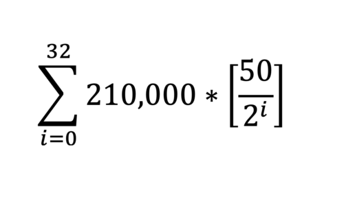
Figure 1. The Bitcoin Supply Formula
If you didn’t study mathematics at school, or it has been some time since you did, at first glance, this Bitcoin supply formula may look confusing or even a little intimidating. We are here today to break down each part and explain exactly what is going on within this famous formula.
As alluded to above, within this formula exist some key numbers related to how the Bitcoin protocol functions.
Let’s introduce these concepts, and these numbers and what they mean (Figure 2). We will study these individual ingredients before throwing them together to bake ourselves the cake that is the Bitcoin Supply Formula.
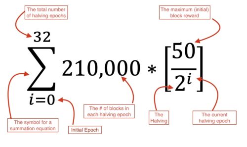
Figure 2. Breaking down the formula
The Math
The Bitcoin supply formula is a mathematical function known as a summation equation? What the hell is a summation equation? It’s simply a series of “+” sums. Let’s introduce some math terms and then continue with a simple exampleto illustrate:
Summation Equations and Limits?
∑ (Sigma) – The Sigma symbol (∑) is the mathematical symbol for summation. This symbol is usually communicated within what we call limits.
The Limits – as mentioned above, these limits, as they relate to our summation equation, are mathematical instructions telling us the boundaries we need to work within for our math problem.. In this case those limits are between i=0 through to and including i=32. Confused? I’ll explain below.
To demonstrate these new consepts of Summation Equations and Limits, let us start with a series of simple equations.
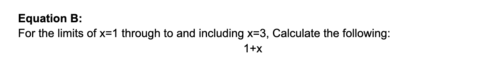
Conduct the following equations:
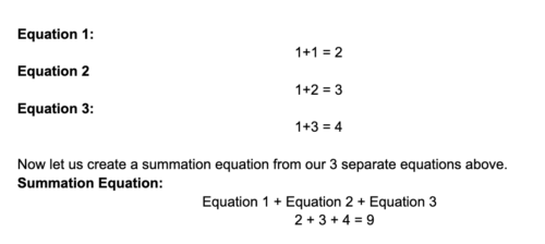
A summation equation is as simple as what we have outlined above. A series of individual equations all added up together at the end.
But how could we represent and communicate this better, rather than having to type out 3 separate equations?
Let’s use Algebra.
I know, I know, for some of you, the word Algebra is enough to make you break out in pimples while triggering high anxiety levels as you recall sweating over your Year 10 final math exam.
Honestly, algebra is not that scary, it is simply using letters to define a number, usually described as a variable. A variable is just a number that we don’t know the value of, or a number that may “vary”.
In our equations examples above, let’s replace the second number in the equations with the letter “x”, and make one equations and call it Equation A.
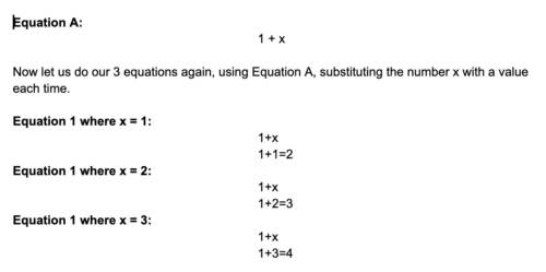
In these quesitons, x was the variable, and its value varied in each equation.
Now, surely we can communicate what we wanted to achieve above even more succinctly?
We can, by using the concept we introduced earlier called limits. Let’s create a new eqaution and spell out what we mean.
With this equation, we simply go through and do exactly like we did above in Equation A, for each value of x, defined within the limits 1 to 3. It is simply a different way of communiciting what we want to achieve.
We can communicate this even more simply using math notation. It actually looks like this.
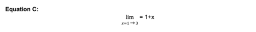
Equation C is effecitvely saying: “I have 3 equations I want you to do. 1 equation for when x=1, another for when x=2 and lastly, another when x=3. And the I want you to perform is 1+x.”
But this only tells us that we want to do 3 separate equations. What It doesn’t tell us yet is that that we want to add them all up at the end.
So, how do we communicate using math notation that we want you to add them all up too? We use the summation equation symbol Sigma (∑).
When we use a Summation Equation, combined with Limits. The notation looks like this:
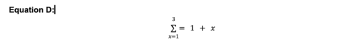
This means, do the calculation 1 + x, substitute the value for x each time, incrementing the value for x each time from 1 through to and including 3, and add up all the answers at the end.
We end up with a single, nice, neat looking equation to communicate what was 3 separate equations at the start, with a final equation to add all 3 up.
See, isn’t math beautiful? From what started looking a little scary and antimidating, ended up being just a series of simple plus(+) sums.
Now that we have a good understanding of the symbols and math notation used in the Bitcoin Supply Formula, let’s look at the individual numbers within the equation and give some colour around what they mean. Don’t worry if you get lost at first. We promise it all comes together at the end.
- i=0 – This is the lower limit of the equation. It represents the inital the initial epoch of time. When the bitcoin protocol was first discovered, we were in the first epoch, when i=0. For each halving epoch, i is incremented +1.
- 32 – 32 is the upper limit for the equation. 32 indicates the total number of halving epochs that will occur within the Bitcoin protocol. For each halving period, i is incremented from 0 (the lower limit) through to and including 32 (the upper limit)
- 210,000 – 210,000 is a function of the supply issuance of new bitcoin, which coincides with the number of blocks each halving. Each period of 210,000 blocks is referred to as one epoch. After each epoch of 210,000 blocks, the summation equation limit (i) is increased +1. The Bitcoin protocol is specifically designed to control the rate of release of new blocks to an average of one block every 10mins. It therefore takes around ~4years (210,000 x 10mins) for each epoch of 210,000 blocks.
- 50 – The initial block reward during the first epoch of Bitcoin’s history was 50. However, as we will see soon, this number is halved during each epoch.
- 2 – This number is how we obtain the term “halving”. At the end of each epoch, the block reward is divided by 2, in other words… it halves.
- “i” = As mentioned above, throughout the summation equation, i is incremented to within the limits of the summation equations and to coincide with the current epoch. During the first epoch, i was 0 and the equation is performed. During the second epoch, i is 1 and the equation is performed again. When we substitute i into the equation, it acts as the exponent of the number 2. Whoa!! Enough math terms already. An exponent is another term for power. Example: When i = 3, within the equation we now see 2^3, which basically means 2 to the power of 3, otherwise 2 x 2 x 2. Similarly, if i were equal to 4, it becomes 2 to the power of 4 (2^4). Which is another way of saying 2 multipled by itself 4 times, e.g 2 x 2 x 2 x 2. The exponent, therefore directly affects the halving intital block reward by (which was initially 50) each epoch by acting as the exponent on the number 2.
With all that laid out, let’s put it all together.
Doing the Math – The Bitcoin Supply Formula.
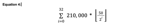
To perform our summation equation, we will do as we did in our earlier examples. We will conduct all of our equations within the limits i=0 through to and including 32. Then add them all up at the end. Revisiting the formula again:
For the first pass, we substitute i=0 into the equation to the right of the Sigma (∑), complete the equation and record your answer.
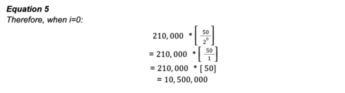
The answer to this calculation corresponds to the total bitcoin supply issuance during the first epoch of Bitcoin’s existence (when i=0). 10,500,00 bitcoin were released as rewards to those who chose to point their computational power toward building and securing the Bitcoin Timechain.
Now, following the rules of the summation equation, once the bitcoin timechain reached a block height of 210,000 blocks (known as Block-Height), the protocol incremented the value of “i” to coincide with the next epoch (when i=1), and we do the equation again, adding it to our existing record.
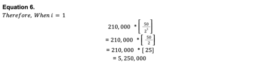
As we can see above, during the second epoch, where i=1, given that the block reward declined from 50 in the first epoch (when i=0) to 25 during the second epoch (when i=1), only 5,250,000 bitcoin were mined
We can now add the supply issuance from both epochs to see how many bitcoin were in circulation after the second epoch.
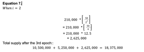
As we move into the 3rd epoch, we simply increment i by +1 and do the equation again and continue to add our totals from each epoch calculation as we go.
By now we should start to see the pattern, as we transition into each epoch, i is incremented by +1 and we do the calculation of issuance for each epoch of 210,000 blocks.
We should now also begin to understand how the block reward is halved each time that i is incremented. We went from a block reward of 50 during the first epoch, to 25 in the second, to 12.5 in the 3rd. And this will continue until the final epoch when i=32.
Each epoch the block rewards are halved. Thus how we coined (pun intended) the term halving. As we continue on each epoch the exponent “i” in the equation will continue to act upon the block reward, halving it each time until we reach the upper limit of our summation equation, when i=32.
Now, we can continue to do each equation one at a time, calculating our results until we reach the final epoch with the upper limit of i=32. We could continue to do this manually, or we could use a calculator, excel sheet or online math tool to do the heavy lifting.
To demonstrate, let’s use excel to do the rest of our work (Figure 3).
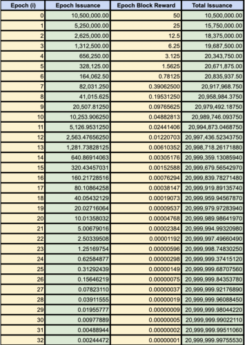
Figure 3. Excel epoch calculations.
Studying the numbers from Figure 3 you might notice something. We often talk about bitcoin as having a fixed supply cap of 21,000,000 bitcoin. If you take the time to do the calculations however, we can see that, actually, we never quite get there. We arrive just short of 21,000,000 by around ~244,470sats.
Hopefully, you now have a better understanding of how the Bitcoin Supply Formula works and maybe even dusted off a few math cobwebs along the way.
For a deeper dive into the mechanics behind Bitcoin, we highly recommend you check out our book: B is for Bitcoin available in both print and ebook formats via Amazon.
Thanks for reading
Looking Glass
The Future Is Bright.